Capitolo 20 Alberi di Regressione (Regression Tree: RTREE)
20.1 Introduzione
I metodi basati su albero differiscono dai metodi di regressione perché partizionano lo spazio delle feature in un insieme di regioni rettangolari, e quindi adattano un modello semplice (una cosrante) in ciacuna regione. Questi sono concettualmente semplici ma potenti. Descriviamo ora un metodo per la regressione e classificazione basata su albero chiamata CART.
20.2 Esempio: package rpart
Illustriamo ora l’idea sottostante agli alberi di regressione che usano dati su marche di
automobili presi dal package rpart.
rpart calcola la media entro i nodi degli alberi.
Consideriamo il data set cu.summary del package rpart.
Facciamo dapprima “crescere” l’albero
di un modello ad albero di regressione in cui Mileage dipende
dalle variabili Country, Reliability Type:
fit <- rpart(Mileage ~ Price + Country + Reliability + Type, method = "anova",
                         data = cu.summary, control = rpart.control(cp = 0.001))
printcp(fit)    # mostra i risultati
##
## Regression tree:
## rpart(formula = Mileage ~ Price + Country + Reliability + Type,
## data = cu.summary, method = "anova", control = rpart.control(cp = 0.001))
##
## Variables actually used in tree construction:
## [1] Price Type
##
## Root node error: 1354.6/60 = 22.576
##
## n=60 (57 observations deleted due to missingness)
##
## CP nsplit rel error xerror xstd
## 1 0.622885 0 1.00000 1.00994 0.174000
## 2 0.132061 1 0.37711 0.52262 0.101517
## 3 0.025441 2 0.24505 0.36907 0.080615
## 4 0.011604 3 0.21961 0.38624 0.081913
## 5 0.001000 4 0.20801 0.41650 0.082874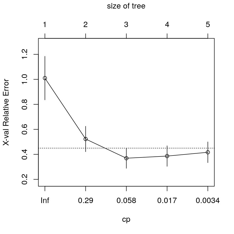
## Call:
## rpart(formula = Mileage ~ Price + Country + Reliability + Type,
## data = cu.summary, method = "anova", control = rpart.control(cp = 0.001))
## n=60 (57 observations deleted due to missingness)
##
## CP nsplit rel error xerror xstd
## 1 0.62288527 0 1.0000000 1.0099426 0.17399960
## 2 0.13206061 1 0.3771147 0.5226204 0.10151732
## 3 0.02544094 2 0.2450541 0.3690684 0.08061485
## 4 0.01160389 3 0.2196132 0.3862442 0.08191343
## 5 0.00100000 4 0.2080093 0.4165042 0.08287384
##
## Variable importance
## Price Type Country
## 48 42 10
##
## Node number 1: 60 observations, complexity param=0.6228853
## mean=24.58333, MSE=22.57639
## left son=2 (48 obs) right son=3 (12 obs)
## Primary splits:
## Price < 9446.5 to the right, improve=0.6228853, (0 missing)
## Type splits as LLLRLL, improve=0.5044405, (0 missing)
## Reliability splits as LLLRR, improve=0.1263005, (11 missing)
## Country splits as --LRLRRRLL, improve=0.1243525, (0 missing)
## Surrogate splits:
## Type splits as LLLRLL, agree=0.950, adj=0.750, (0 split)
## Country splits as --LLLLRRLL, agree=0.833, adj=0.167, (0 split)
##
## Node number 2: 48 observations, complexity param=0.1320606
## mean=22.70833, MSE=8.498264
## left son=4 (23 obs) right son=5 (25 obs)
## Primary splits:
## Type splits as RLLRRL, improve=0.43853830, (0 missing)
## Price < 12154.5 to the right, improve=0.25748500, (0 missing)
## Country splits as --RRLRL-LL, improve=0.13345700, (0 missing)
## Reliability splits as LLLRR, improve=0.01637086, (10 missing)
## Surrogate splits:
## Price < 12215.5 to the right, agree=0.812, adj=0.609, (0 split)
## Country splits as --RRLRL-RL, agree=0.646, adj=0.261, (0 split)
##
## Node number 3: 12 observations
## mean=32.08333, MSE=8.576389
##
## Node number 4: 23 observations, complexity param=0.02544094
## mean=20.69565, MSE=2.907372
## left son=8 (10 obs) right son=9 (13 obs)
## Primary splits:
## Type splits as -LR--L, improve=0.515359600, (0 missing)
## Price < 14962 to the left, improve=0.131259400, (0 missing)
## Country splits as ----L-R--R, improve=0.007022107, (0 missing)
## Surrogate splits:
## Price < 13572 to the right, agree=0.609, adj=0.1, (0 split)
##
## Node number 5: 25 observations, complexity param=0.01160389
## mean=24.56, MSE=6.4864
## left son=10 (14 obs) right son=11 (11 obs)
## Primary splits:
## Price < 11484.5 to the right, improve=0.09693168, (0 missing)
## Reliability splits as LLRRR, improve=0.07767167, (4 missing)
## Type splits as L--RR-, improve=0.04209834, (0 missing)
## Country splits as --LRRR--LL, improve=0.02201687, (0 missing)
## Surrogate splits:
## Country splits as --LLLL--LR, agree=0.80, adj=0.545, (0 split)
## Type splits as L--RL-, agree=0.64, adj=0.182, (0 split)
##
## Node number 8: 10 observations
## mean=19.3, MSE=2.21
##
## Node number 9: 13 observations
## mean=21.76923, MSE=0.7928994
##
## Node number 10: 14 observations
## mean=23.85714, MSE=7.693878
##
## Node number 11: 11 observations
## mean=25.45455, MSE=3.520661Nota: \(R_{cp}(T) = R(T) + cp * |T| * R(T_0)\) cioè: se un qualunque split non incrementa l’\(R^2\) complessivo del modelo di una quantità almeno pari a \(cp\) (dove \(R^2\) in questo caso è il classico coefficiente di determinazione dei modelli lineari) allora questo split verrà dichiarato essere, a priori, non migliorativo. Possiamo generare dei grafici aggiuntivi:
##
## Regression tree:
## rpart(formula = Mileage ~ Price + Country + Reliability + Type,
##     data = cu.summary, method = "anova", control = rpart.control(cp = 0.001))
##
## Variables actually used in tree construction:
## [1] Price Type
##
## Root node error: 1354.6/60 = 22.576
##
## n=60 (57 observations deleted due to missingness)
##
##         CP nsplit rel error  xerror     xstd
## 1 0.622885      0   1.00000 1.00994 0.174000
## 2 0.132061      1   0.37711 0.52262 0.101517
## 3 0.025441      2   0.24505 0.36907 0.080615
## 4 0.011604      3   0.21961 0.38624 0.081913
## 5 0.001000      4   0.20801 0.41650 0.082874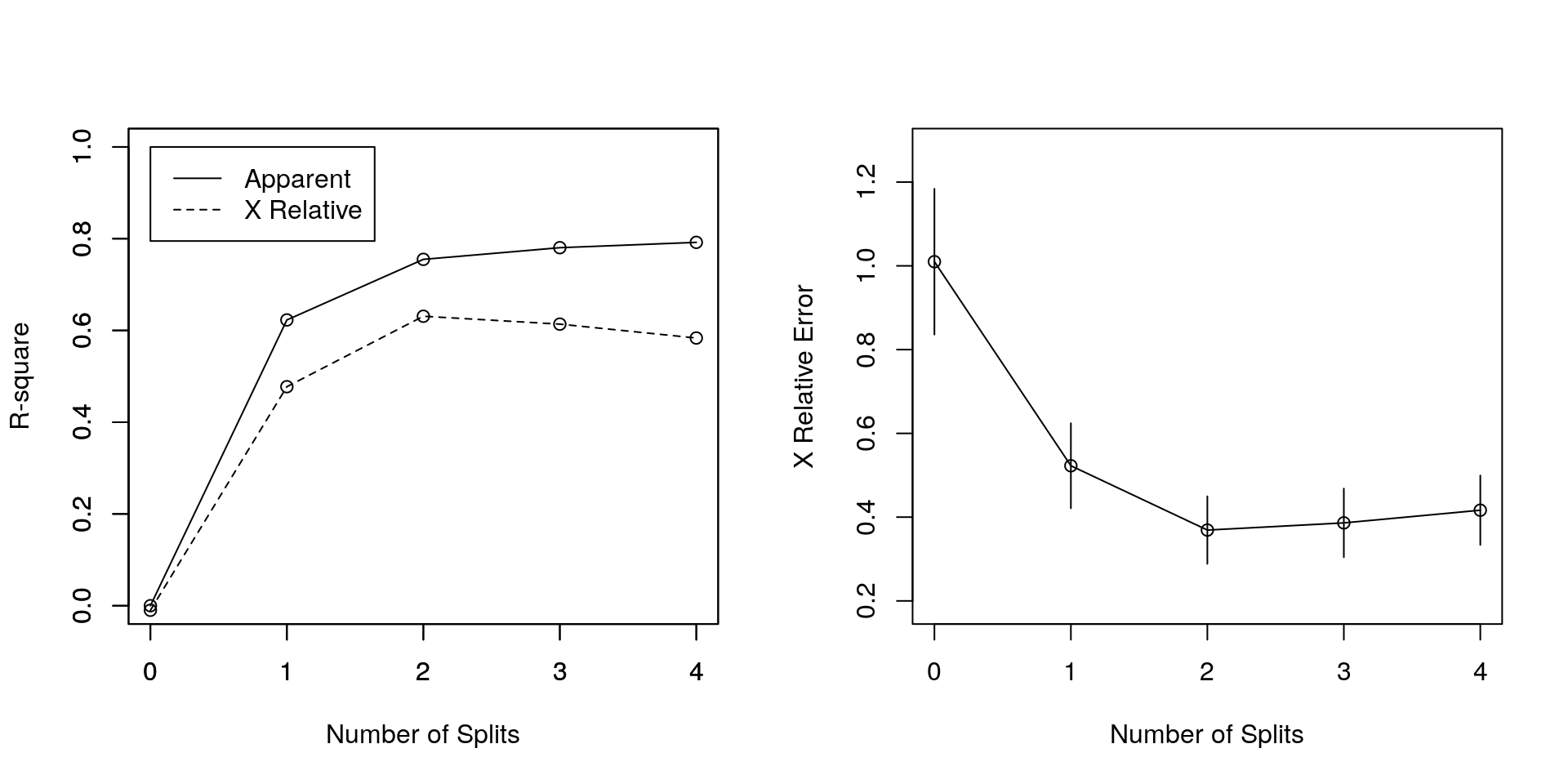
Il valore di X Relative Error è collegabile ai valori dei residui PRESS.
Infine rappresentiamo graficamente l’albero:
plot(fit, uniform = TRUE, main = "Albero di regressione per Mileage")
text(fit, use.n = TRUE, all = TRUE, cex = .8)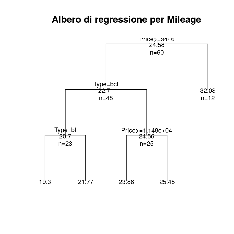
Ed ora potiamo l’albero in corrispondenza del valore di cp “ottimo”:
Ora possiamo tracciare nuovamente l’albero, questa volta potato:
plot(pfit, uniform = TRUE, main = "Albero di regressione potato per Mileage")
text(pfit, use.n = TRUE, all = TRUE, cex = .8)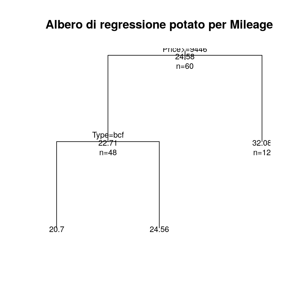
Che ritorna un albero più semplice rispetto all’originale.
20.3 Esempio: package party
Come esempio finale, vorrei mostrare il package party, la cui funzione mob()
implementa una variante dell’approccio degli alberi di regressione descritti finora
chiamata partizionamento ricorsivo model-based (model-based recursive partitioning).
La funzione mob() permette di stimare modelli di regressione separati, spezzando
i dati tramite alcune variabili. La formula per specificare tale modello è:
y ~ x1 + x2 + … + xk | z1 + … + zl,
dove i termini alla sinistra del | specificano le variabili di regressione,
mentre i termini alla destra del | specificano le variabili per il partizionamento. La
procedura generale per l’adattamento è la seguente:
- Adatta il modello una volta su tutte le osservazioni nel nodo corrente.
- Valuta se le stime dei parametri sono stabili rispetto a tutte le varibili di partizionamento z1, . . . , zl. Se c’è qualche instabilità, seleziona per il partizionamento la variabile zj associata con il più piccolo p-value; altrimenti fermati.
- Calcola i punti di split che ottimizzano localmente una funzione obiettivo.
- Riadatta il modello in entrambi i figlio, e ritorna al passo 2.
A scopo illustrativo, consideriamo un esempio basato sul ben noto dataset bostonhousing.
Questo dataset contiene informazioni per 506 case di Boston. In particolare, il dataset fornisce il valore mediano delle case (in migliaia di USD) insieme a 14 covariate, tra cui il numero di camere per abitazione (rm) e la percentuale di popolazione con stato economico basso (lstat).
Una relazione a segmenti tra il valore delle case e queste due variabili risulta molto intuitivo, mentre la forma dell’influenza delle rimanenti covariate è poco chiara e dovrebbe quindi essere appresa dai dati. Di conseguenza, è utilizzato un modello di regressione lineare per il valore mediano spiegato da rm^2 e log(lstat) con k = 3 coefficienti di regressione, e con un partizionamento rispetto alle l = 11 variabili rimanenti.
bostonhousing$lstat <- log(bostonhousing$lstat)
bostonhousing$rm <- bostonhousing$rm^2
bostonhousing$chas <- factor(bostonhousing$chas, levels = 0:1, labels = c("no", "yes"))
bostonhousing$rad <- factor(bostonhousing$rad, ordered = TRUE)
Entrambe le trasformazioni impattano solo sui test di stabilità dei parametri (step 2), ma non sulla procedura di splitting (step 3).
Carichiamo il package party, che permette l’analisi
E impostiamo alcuni parametri di controllo per la procedura:
ctrl <- mob_control(alpha = 0.05, bonferroni = TRUE,
                    minsplit = 40, objfun = deviance,
                    verbose = TRUE)
Ora possiamo stimare e visualizzare il modello:
fmBH <- mob(medv ~ age + lstat + rm | zn + indus + chas + nox + age + dis + rad + tax + crim + b + ptratio,
            data = bostonhousing, control = ctrl, model = linearModel)
##
## -------------------------------------------
## Fluctuation tests of splitting variables:
## zn indus chas nox age
## statistic 3.915651e+01 6.48353e+01 20.144236012 9.483200e+01 3.203777e+01
## p.value 2.748895e-05 7.27457e-11 0.005144677 1.155427e-17 7.976832e-04
## dis rad tax crim b
## statistic 6.984690e+01 1.200538e+02 9.282845e+01 8.822816e+01 3.344074e+01
## p.value 5.503655e-12 4.493345e-11 3.329097e-17 3.759587e-16 4.150856e-04
## ptratio
## statistic 7.722485e+01
## p.value 1.195801e-13
##
## Best splitting variable: nox
## Perform split? yes
## -------------------------------------------
##
## Node properties:
## nox <= 0.597; criterion = 1, statistic = 120.054
##
## -------------------------------------------
## Fluctuation tests of splitting variables:
## zn indus chas nox age
## statistic 22.16164033 38.155039447 13.1622614 3.613344e+01 21.19908930
## p.value 0.06002158 0.000042868 0.1097181 1.119481e-04 0.08950553
## dis rad tax crim b
## statistic 4.984273e+01 7.873614e+01 5.664802e+01 3.832894e+01 16.1842317
## p.value 1.439457e-07 8.981811e-05 4.795733e-09 3.945393e-05 0.4811923
## ptratio
## statistic 4.680235e+01
## p.value 6.464767e-07
##
## Best splitting variable: tax
## Perform split? yes
## -------------------------------------------
##
## Node properties:
## tax <= 265; criterion = 1, statistic = 78.736
##
## -------------------------------------------
## Fluctuation tests of splitting variables:
## zn indus chas nox age dis rad
## statistic 3.3545026 10.0069447 5.7151219 3.1451982 7.9081059 7.8745370 26.9826810
## p.value 0.9999773 0.5514421 0.9363047 0.9999919 0.8314404 0.8352436 0.7990803
## tax crim b ptratio
## statistic 5.0300885 16.99327331 5.7652226 14.0764807
## p.value 0.9953639 0.05201363 0.9823021 0.1528855
##
## Best splitting variable: crim
## Perform split? no
## -------------------------------------------
##
## -------------------------------------------
## Fluctuation tests of splitting variables:
## zn indus chas nox age
## statistic 21.5050525 27.142939062 20.926287619 3.319160e+01 13.7113428
## p.value 0.0674627 0.005976414 0.003602557 3.839128e-04 0.7553577
## dis rad tax crim b
## statistic 3.538273e+01 9.122327e+01 25.03035134 30.860920339 15.0157784
## p.value 1.382702e-04 1.475737e-06 0.01509699 0.001121331 0.5826294
## ptratio
## statistic 3.667774e+01
## p.value 7.520021e-05
##
## Best splitting variable: rad
## Perform split? yes
## -------------------------------------------
##
## Splitting ordered factor variable, objective function:
## 1 2 3 4 5 6 7 8
## Inf Inf Inf 2187.271 2276.856 2246.727 2212.269 Inf
##
## Node properties:
## rad <= 4; criterion = 1, statistic = 91.223
##
## -------------------------------------------
## Fluctuation tests of splitting variables:
## zn indus chas nox age
## statistic 21.78717354 25.236137411 4.070877e+01 3.461621e+01 12.3419838
## p.value 0.02779648 0.006848526 3.396900e-07 1.312167e-04 0.6403411
## dis rad tax crim b
## statistic 26.876132486 33.584875615 26.618948311 28.795057224 11.40741
## p.value 0.003476391 0.008624286 0.003868135 0.001559656 0.76027
## ptratio
## statistic 20.62785834
## p.value 0.04411343
##
## Best splitting variable: chas
## Perform split? yes
## -------------------------------------------
##
## Splitting factor variable, objective function:
## no
## Inf
##
## No admissable split found in 'chas'
##
## -------------------------------------------
## Fluctuation tests of splitting variables:
## zn indus chas nox age dis
## statistic 13.6090429 12.3198115 2.5872912 16.2352068 2.022037 13.8616530
## p.value 0.6152638 0.7814215 0.9999817 0.3014644 1.000000 0.5814575
## rad tax crim b ptratio
## statistic 29.9508277 14.1489340 5.150212 9.0700832 25.938682323
## p.value 0.1834797 0.5433336 1.000000 0.9911082 0.006939915
##
## Best splitting variable: ptratio
## Perform split? yes
## -------------------------------------------
##
## Node properties:
## ptratio <= 17.4; criterion = 0.993, statistic = 29.951
##
## -------------------------------------------
## Fluctuation tests of splitting variables:
## zn indus chas nox age dis rad
## statistic 10.3524693 6.6496014 0 5.5187764 4.5664607 3.5232716 17.831172
## p.value 0.6868439 0.9878916 NA 0.9987369 0.9999295 0.9999995 0.982799
## tax crim b ptratio
## statistic 6.6496014 5.7350736 6.5775283 5.7670351
## p.value 0.9878916 0.9978913 0.9892259 0.9977337
##
## Best splitting variable: zn
## Perform split? no
## -------------------------------------------
##
## -------------------------------------------
## Fluctuation tests of splitting variables:
## zn indus chas nox age dis
## statistic 21.75804148 20.45640956 4.9569007 22.42659195 5.095982 3.354260e+01
## p.value 0.04436417 0.07545764 0.9775062 0.03365479 1.000000 2.655947e-04
## rad tax crim b ptratio
## statistic 3.498962e+01 3.257007e+01 26.074408168 9.5942144 3.257007e+01
## p.value 2.954067e-04 4.115671e-04 0.007194095 0.9870579 4.115671e-04
##
## Best splitting variable: dis
## Perform split? yes
## -------------------------------------------
##
## Node properties:
## dis <= 1.6074; criterion = 1, statistic = 34.99
##
## -------------------------------------------
## Fluctuation tests of splitting variables:
## zn indus chas nox age dis rad
## statistic 9.5080465 7.3966404 12.9583514 21.92048165 2.18296 6.7267273 23.8624502
## p.value 0.9644422 0.9990245 0.1192863 0.02992438 1.00000 0.9998421 0.0265835
## tax crim b ptratio
## statistic 20.79309498 20.61629801 12.7217188 17.7130063
## p.value 0.04739517 0.05091238 0.6560969 0.1498435
##
## Best splitting variable: rad
## Perform split? yes
## -------------------------------------------
##
## Splitting ordered factor variable, objective function:
## 1 2 3 4 5 6 7 8
## Inf Inf Inf Inf 875.6391 875.6391 875.6391 875.6391
##
## Node properties:
## rad <= 5; criterion = 0.973, statistic = 23.862## 1) nox <= 0.597; criterion = 1, statistic = 120.054
## 2) tax <= 265; criterion = 1, statistic = 78.736
## 3)* weights = 82
## Terminal node model
## Linear model with coefficients:
## (Intercept) age lstat rm
## -2.23429 0.02483 -3.01289 0.81660
##
## 2) tax > 265
## 4) rad <= 4; criterion = 1, statistic = 91.223
## 5)* weights = 111
## Terminal node model
## Linear model with coefficients:
## (Intercept) age lstat rm
## -3.43902 -0.07993 1.06950 0.70388
##
## 4) rad > 4
## 6) ptratio <= 17.4; criterion = 0.993, statistic = 29.951
## 7)* weights = 57
## Terminal node model
## Linear model with coefficients:
## (Intercept) age lstat rm
## 7.731363 -0.006482 -2.864374 0.585465
##
## 6) ptratio > 17.4
## 8)* weights = 91
## Terminal node model
## Linear model with coefficients:
## (Intercept) age lstat rm
## 12.2025 -0.0687 -0.6483 0.3870
##
## 1) nox > 0.597
## 9) dis <= 1.6074; criterion = 1, statistic = 34.99
## 10)* weights = 40
## Terminal node model
## Linear model with coefficients:
## (Intercept) age lstat rm
## 97.1330 -0.1065 -20.6139 -0.2542
##
## 9) dis > 1.6074
## 11) rad <= 5; criterion = 0.973, statistic = 23.862
## 12)* weights = 50
## Terminal node model
## Linear model with coefficients:
## (Intercept) age lstat rm
## 38.3059 -0.1677 -9.2983 0.5834
##
## 11) rad > 5
## 13)* weights = 75
## Terminal node model
## Linear model with coefficients:
## (Intercept) age lstat rm
## 61.34934 -0.09697 -12.19267 -0.06927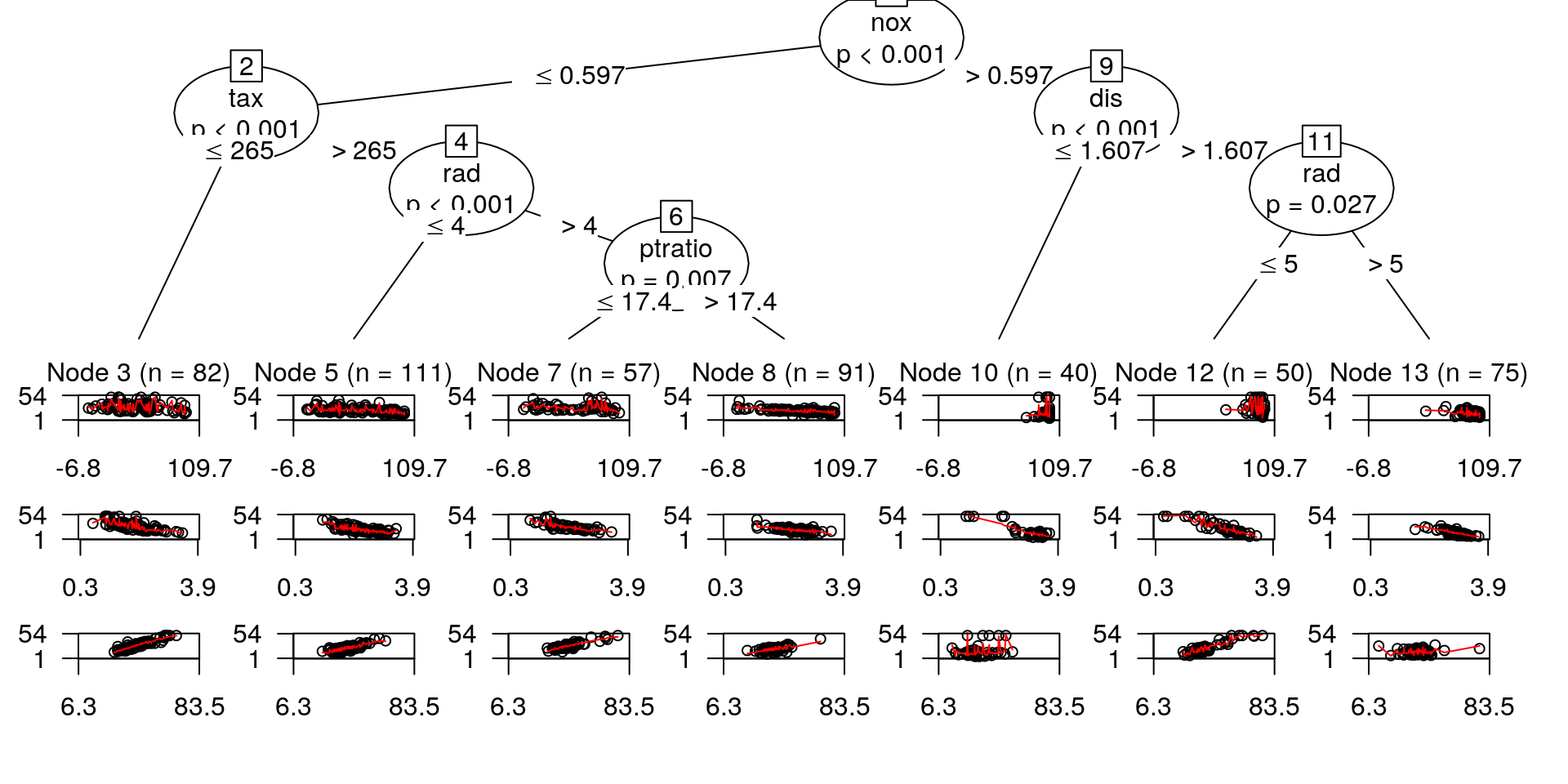
##    (Intercept)          age       lstat          rm
## 3    -2.234289  0.024827161  -3.0128873  0.81659999
## 5    -3.439016 -0.079931189   1.0695002  0.70387750
## 7     7.731363 -0.006482131  -2.8643737  0.58546514
## 8    12.202515 -0.068697423  -0.6483409  0.38703319
## 10   97.133016 -0.106517216 -20.6139361 -0.25421913
## 12   38.305900 -0.167657196  -9.2983159  0.58342155
## 13 61.349342 -0.096967406 -12.1926707 -0.06926919## $`3`
##
## Call:
## NULL
##
## Weighted Residuals:
## Min 1Q Median 3Q Max
## -6.479 0.000 0.000 0.000 12.831
##
## Coefficients:
## Estimate Std. Error t value Pr(>|t|)
## (Intercept) -2.23429 4.26921 -0.523 0.6022
## age 0.02483 0.01983 1.252 0.2143
## lstat -3.01289 1.16980 -2.576 0.0119 *
## rm 0.81660 0.06168 13.240 <2e-16 ***
## ---
## Signif. codes: 0 '***' 0.001 '**' 0.01 '*' 0.05 '.' 0.1 ' ' 1
##
## Residual standard error: 3.18 on 78 degrees of freedom
## Multiple R-squared: 0.8893, Adjusted R-squared: 0.885
## F-statistic: 208.8 on 3 and 78 DF, p-value: < 2.2e-16
##
##
## $`5`
##
## Call:
## NULL
##
## Weighted Residuals:
## Min 1Q Median 3Q Max
## -7.703 0.000 0.000 0.000 7.973
##
## Coefficients:
## Estimate Std. Error t value Pr(>|t|)
## (Intercept) -3.43902 3.75219 -0.917 0.361
## age -0.07993 0.01137 -7.030 2.02e-10 ***
## lstat 1.06950 0.94523 1.131 0.260
## rm 0.70388 0.05563 12.652 < 2e-16 ***
## ---
## Signif. codes: 0 '***' 0.001 '**' 0.01 '*' 0.05 '.' 0.1 ' ' 1
##
## Residual standard error: 2.612 on 107 degrees of freedom
## Multiple R-squared: 0.8034, Adjusted R-squared: 0.7979
## F-statistic: 145.7 on 3 and 107 DF, p-value: < 2.2e-16
##
##
## $`7`
##
## Call:
## NULL
##
## Weighted Residuals:
## Min 1Q Median 3Q Max
## -7.284 0.000 0.000 0.000 8.406
##
## Coefficients:
## Estimate Std. Error t value Pr(>|t|)
## (Intercept) 7.731363 6.026114 1.283 0.2051
## age -0.006482 0.023136 -0.280 0.7804
## lstat -2.864374 1.674810 -1.710 0.0931 .
## rm 0.585465 0.082100 7.131 2.77e-09 ***
## ---
## Signif. codes: 0 '***' 0.001 '**' 0.01 '*' 0.05 '.' 0.1 ' ' 1
##
## Residual standard error: 3.3 on 53 degrees of freedom
## Multiple R-squared: 0.8231, Adjusted R-squared: 0.8131
## F-statistic: 82.22 on 3 and 53 DF, p-value: < 2.2e-16
##
##
## $`8`
##
## Call:
## NULL
##
## Weighted Residuals:
## Min 1Q Median 3Q Max
## -9.303 0.000 0.000 0.000 6.571
##
## Coefficients:
## Estimate Std. Error t value Pr(>|t|)
## (Intercept) 12.20252 4.01279 3.041 0.00312 **
## age -0.06870 0.01638 -4.193 6.59e-05 ***
## lstat -0.64834 1.15267 -0.562 0.57524
## rm 0.38703 0.05936 6.520 4.44e-09 ***
## ---
## Signif. codes: 0 '***' 0.001 '**' 0.01 '*' 0.05 '.' 0.1 ' ' 1
##
## Residual standard error: 2.54 on 87 degrees of freedom
## Multiple R-squared: 0.6675, Adjusted R-squared: 0.6561
## F-statistic: 58.23 on 3 and 87 DF, p-value: < 2.2e-16
##
##
## $`10`
##
## Call:
## NULL
##
## Weighted Residuals:
## Min 1Q Median 3Q Max
## -8.654 0.000 0.000 0.000 19.814
##
## Coefficients:
## Estimate Std. Error t value Pr(>|t|)
## (Intercept) 97.1330 22.5728 4.303 0.000123 ***
## age -0.1065 0.2063 -0.516 0.608780
## lstat -20.6139 1.7396 -11.850 5.53e-14 ***
## rm -0.2542 0.1153 -2.205 0.033922 *
## ---
## Signif. codes: 0 '***' 0.001 '**' 0.01 '*' 0.05 '.' 0.1 ' ' 1
##
## Residual standard error: 6.14 on 36 degrees of freedom
## Multiple R-squared: 0.8059, Adjusted R-squared: 0.7897
## F-statistic: 49.83 on 3 and 36 DF, p-value: 6.747e-13
##
##
## $`12`
##
## Call:
## NULL
##
## Weighted Residuals:
## Min 1Q Median 3Q Max
## -5.745 0.000 0.000 0.000 5.369
##
## Coefficients:
## Estimate Std. Error t value Pr(>|t|)
## (Intercept) 38.30590 5.98897 6.396 7.36e-08 ***
## age -0.16766 0.05205 -3.221 0.00235 **
## lstat -9.29832 0.87606 -10.614 5.92e-14 ***
## rm 0.58342 0.04520 12.908 < 2e-16 ***
## ---
## Signif. codes: 0 '***' 0.001 '**' 0.01 '*' 0.05 '.' 0.1 ' ' 1
##
## Residual standard error: 2.471 on 46 degrees of freedom
## Multiple R-squared: 0.9601, Adjusted R-squared: 0.9575
## F-statistic: 368.9 on 3 and 46 DF, p-value: < 2.2e-16
##
##
## $`13`
##
## Call:
## NULL
##
## Weighted Residuals:
## Min 1Q Median 3Q Max
## -7.532 0.000 0.000 0.000 8.328
##
## Coefficients:
## Estimate Std. Error t value Pr(>|t|)
## (Intercept) 61.34934 4.67059 13.135 < 2e-16 ***
## age -0.09697 0.04014 -2.416 0.0183 *
## lstat -12.19267 1.15276 -10.577 3.1e-16 ***
## rm -0.06927 0.04454 -1.555 0.1243
## ---
## Signif. codes: 0 '***' 0.001 '**' 0.01 '*' 0.05 '.' 0.1 ' ' 1
##
## Residual standard error: 2.894 on 71 degrees of freedom
## Multiple R-squared: 0.6859, Adjusted R-squared: 0.6727
## F-statistic: 51.69 on 3 and 71 DF, p-value: < 2.2e-16Per riepilogare la qualità del modello, possiamo calcolare il mean squared error, la log-verosimiglianza e l’indice AIC:
## [1] 9.664305## 'log Lik.' -1255.384 (df=41)## [1] 2592.768